12 ShinyApps
By Poppy Riddle
12.1 Learning objecives
In this chapter, we’ll be looking in more detail at the input and output functions using examples. This chapter introduces you to:
input functions for text, numbers, dates, choices, file uploads and actions,
output functions for text, tables, plots, images, and download formats,
an introduction to themes to change the appearance of your application, and
an explanation of reactivity and how its used.
We’ll be using some of the dataset standards included in R, such as mtcars and iris, as example datasets. Feel free to explore the datasets on your own, or even replace with your own data as you play with these inputs.
You can see all the datasets included in R by typing data() in the console.
You may also find the RStudio and Shiny cheatsheets helpful.
12.2 Inputs & Widgets
Inputs are the ways users can enter, filter, or select information within your app. Widgets are a type of input that requires a different mode of input than text, such as a slider or button. There is a basic format to the inputs & widgets. First there is the input type, in this case, a textAreaInput(). In the first position is the inputID parameter, followed by the label parameter. These two will be consistent with all inputs. After the inputID and the label, arguments that may be unique to each follow. In this case, there is an argument for the number of rows. In general, all inputs, (including widgets) keep this order of inputID, label, arguments.
textAreaInput("story", "Tell me about yourself", rows = 3)While we will address a few of these, you can find all of them and their code on the shiny gallery.
The syntax of the widget is the same as other inputs. Let’s look at the code below:
The inputID has some rules, just like any variable in R. It must be:
First, a string consisting of letters, numbers, and/or underscores. Other characters like spaces, symbols, dashes, periods, etc., won’t work.
Second, it must be unique as you will call this in output functions.
You can find all of these in the input section in the shiny references documentation here. The following selection are some of the more commonly used ones to get you started. Inputs and outputs will be shown in context of the ui or server component. You can build an app as you go along. You may want to start with the basic structure first and try different inputs as your read through the chapter.
library(shiny)

ui <- fluidPage(

)#close fluidPage

server <- function(input, output) {

} #close server function

shinyApp(ui, server)If you ever want to know more about a function, you can always use the help section in RStudio or use the console to place a ? before the function, such as ?fluidPage.
12.2.1 Text input
12.2.1.0.1 textInput()
This is for small amounts of text, like asking for someone’s name, address, or what type of donut they like. You can find the documentation on this input here. To format text, for size, emphasis, color, etc, please see the Formatting text section at the end of the Outputs section.
ui <- fluidPage(
  textInput("input_1", "What's your favorite donut?"),
  )#close fluidPage
12.2.1.0.2 passwordInput()
This is for entering passwords. You can find more info here on its arguments.
ui <- fluidPage(
  textInput("input_1", "What's your favorite donut?"),
  passwordInput("pword_1", "If a donut was your password, what would it be?")
)#close fluidPage
12.2.1.0.3 textAreaInput()
This one is better for longer sections of text, like bio’s for websites, brief passages, comments, special instructions, etc. You can find more info here on its arguments.
ui <- fluidPage(
  textInput("input_1", "What's your favorite donut?"),
  passwordInput("pword_1", "If a donut was your password, what would it be?"),
  textAreaInput("bio", "Please describe yourself as a donut", rows = 3)

)#close fluidPage
So, let’s see these inputs as a complete application.
library(shiny)

ui <- fluidPage(
  textInput("input_1", "What's your favorite donut?"),
  passwordInput("pword_1", "If a donut was your password, what would it be?"),
  textAreaInput("bio", "Please describe yourself as a donut", rows = 3)
)#close fluidPage

server <- function(input, output){
}

# Run the application
shinyApp(ui = ui, server = server)
12.2.2 Number inputs
Here are three inputs for numbers. You can find documentation here for the arguments.
12.2.2.0.1 numericInput()
ui <- fluidPage(
  numericInput("num_1", "Enter the quantity of donuts", value = 0, min = 0, max = 12)
)#close fluidPage
12.2.2.0.2 sliderInput()
Slider inputs can be used to select a single number or specify a range. Note the list argument passed in the second sliderInput() function named num_3. Documentation is here.
ui <- fluidPage(
  sliderInput("num_2", "Enter the maximum number you can eat in one go", value = 6, min = 0, max = 12),
  sliderInput("num_3", "Enter the range of donuts you have been known to eat", value=c(3,9), min=0, max=12 )
)#close fluidPage
12.2.2.0.3 dateInput() and dateRangeInput()
For single date entry, use the dateInput() function. For a range of dates, use the dateRangeInput(). Easy, right? There are format options for date inputs, such as format, language, and value which defines the starting date. The default starting date is today’s date on your system. You can use the help section to find out more or the documentation here for dateInput() and here for dateRangeInput().
ui <- fluidPage(
  dateInput("order_1", "What date do you want to order donuts?"),
  dateRangeInput("delivery_1","Between what dates do you want the donuts delivered?")

)#close fluidPage
12.2.3 Choices from a list
12.2.3.0.1 selectInput()
This provides a drop down list based on a list. In the following example, the list has been defined first, but this list could also be passed within the selectInput() function.
flavors <- c("chocolate", "plain", "raspberry", "maple", "unicorn", "creme-filled", "sprinkles", "chef's choice")

ui <- fluidPage(
  selectInput("flavor_1", "What flavor of donut would you like?", flavors, multiple=TRUE)

)#close fluidPage12.2.3.0.3 checkboxInput() and checkboxGroupInput()
An alternative to radio buttons is check boxes which can be used for lists, surveys, or yes/no decions. For checkboxInput(), the value argument is a boolean TRUE or FALSE that determines if its automatically checked. checkboxGroupInput() also lets you select multiple choices, which the radio button does not.
flavors <- c("chocolate", "plain", "raspberry", "maple", "unicorn", "creme-filled", "sprinkles", "chef's choice")

ui <- fluidPage(
  checkboxInput("choice_1", "Eat here", value=TRUE),
  checkboxInput("choice_2", "Take home"),
  checkboxGroupInput("multiple_choice", "What flavors would you like?", flavors, selected = NULL)

)#closed fluidPageBy now, you should be using the ?function, (such as ?checkboxGroupInput) in the console or searching for the function in the help page, (usually on the right in RStudio). Or use cheatsheets such as this one for shiny. This is a normal part of workflow and will help you add arguments to control input behaviours.
12.3 Outputs
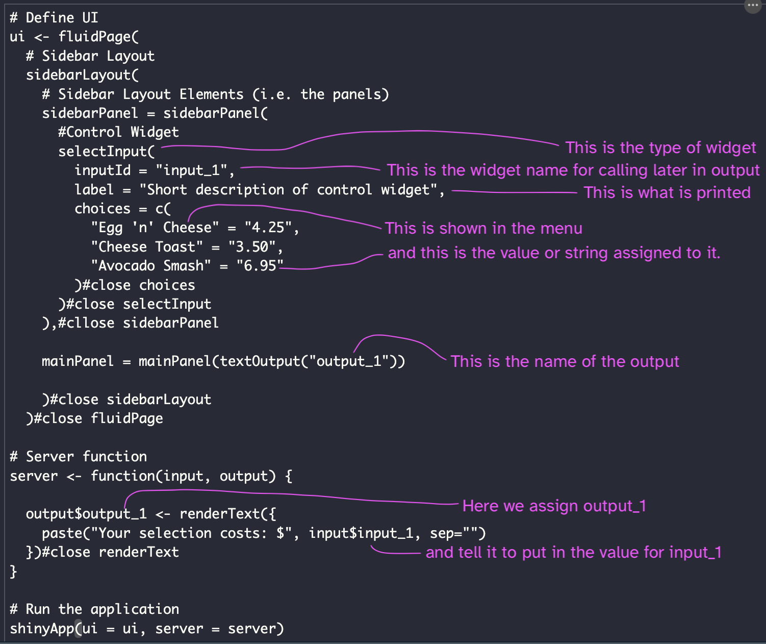
Outputs are paired functions with one assigned in the ui to define spaces where outputs will be seen and the other in the server function to render the result. They include a unique ID in the first position of its arguments.
Output ID’s are called from the server side preceded by output$outputID in which outputID is the ID (like a variable name) you’ve assigned it. You’ll see these are always calling a render* function, such as renderText(). As an example:
Some important new fuctions are called. In the server() function, you see renderText(). This calls the values you assigned in input_1 and places it where you assigned it in output_1. In addition to text, you can also render tables, data tables, plots, images, and text. *Output() and render*() functions work together, with *Output() in the ui to show where output will be displayed, and render*() in the server to produce the desired information.
12.3.1 Text output
12.3.1.0.1 textOutput() & renderText()
This outputs regular text. You can see the placeholder textOutput() in the ui, and the renderText() function passed in the server. Here, we use the input of input_1 as the output for text.
library(shiny)
ui <- fluidPage(
textInput("input_1", "What's your favorite donut?"),
h4("Your favorite donut is: "),
textOutput("text")
)#close fluidPage
server <- function(input, output) {
output$text <- renderText({input$input_1})
}#close server
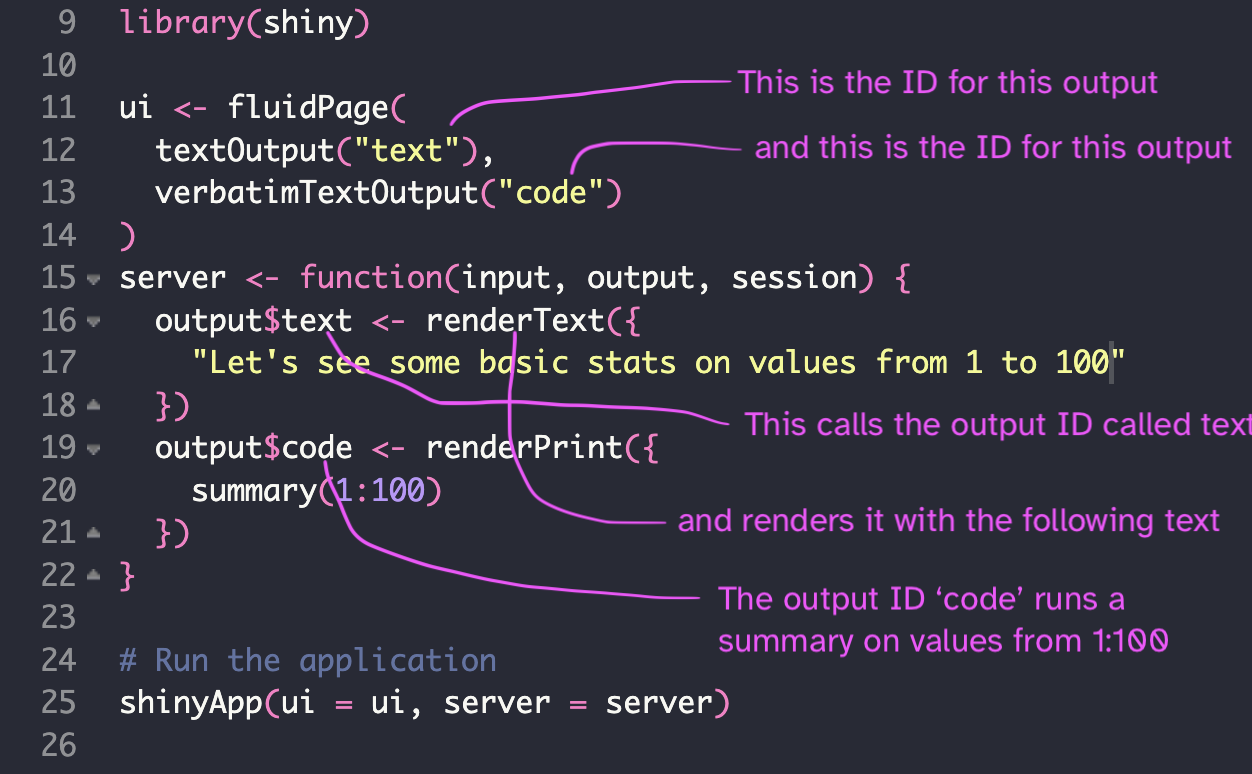
shinyApp(ui, server)12.3.1.0.2 verbatimTextOutput() & renderPrint()
This creates a console like output in the application. Lets add the dataset summary. renderPrint() prints the results of expressions, where renderText() prints text together in a string.
ui <- fluidPage(
  textOutput("text"),
  verbatimTextOutput("code")

)#close fluidPage

server <- function(input, output) {
  output$text <- renderText({
    "Hello. The following is a summary of a standard R dataset, mtcars"
  })
  output$code <- renderPrint({
    summary(mtcars)
  })
}#close server
12.3.2 Tables
Oh, tables! Tables are powerful. There are two types of tables, static tables of data, and dynamic tables that are interactive.
12.3.2.0.1 tableOutput() & renderTable()
Static tables are great for summaries or concise results. They’re good at preserving data just the way you made it.
ui <- fluidPage(
  tableOutput("static")
)#close fluidPage

server <- function(input, output) {
  output$static <- renderTable(head(mtcars))
}#close server
12.3.2.0.2 dataTableOutput() & renderDataTable()
DataTables are much more dynamic and can be customized in numerous ways.
ui <- fluidPage(
  dataTableOutput("dynamic")

)#close fluidPage

server <- function(input, output) {
  output$dynamic <- renderDataTable(mtcars, options=list(pageLength = 6)
  )#cloe renderDataTable
}#close server
DataTables are more appropriate for larger dataframes where someone may need to explore, filter, and sort data. You can find more information on modifying DataTables here.
DataTables refers to both functions in Shiny and from the DT library. Unless the library(DT) is called, references to dataTables are for the version in the Shiny library. While dataTables in the Shiny library provides only server-side tables, the DT package can provide both server-side and client-side tables. This may be an important consideration if you are trying to reduce how many working hours your application runs on shinyapps.io, for example.
12.3.3 DataTables
In this section, we are going to explore importing data and displaying it in a DataTable using the DT library. This is different than the data.table function included in the Shiny library. The DT library makes a lovely table that can be searched, filtered, and sorted which is great for data exploration. You can find more info here and here for the DT documentation.
library(shiny)
library(DT)

ui <- fluidPage(
  h2("Some data about flowers"),
  DT::dataTableOutput("table_1")

)#close fluidPage

server <- function(input, output) {
  output$table_1 = DT::renderDataTable({
  iris
  })#close output

}#close server

shinyApp(ui, server)You can in the code above that the DT library has been called. Its also good practice to call directly from the library for functions that are present in more than one library. In this case, renderDataTable() exists in both Shiny and DT. To make it more human readable and prevent conflicts, its advised to call the function directly from the library as in the following:
DT::renderDataTable()
12.3.4 Computation output
But what if we wanted to perform some operations on the data, such as to use the summarizing functions you did in earlier chapters on the mtcars dataset? In the code below, we first import some data from a remote location, then create a DataTable for exploration. Then we summarize the data.
library(shiny)
library(DT)
library(tidyverse)


path <- "https://raw.githubusercontent.com/fivethirtyeight/data/master/comic-characters/marvel-wikia-data.csv"

# This will read the first sheet of the Excel file
comics_data <- read_csv(path)

ui <- fluidPage(
  sidebarLayout(
    sidebarPanel(
      h2("How to use DataTables from the DT library"),
      br(),
      p("To the right is a dataset displayed as a DataTable"),
      p("This dataset is from the fivethirtyeight GitHub repository.")
    ),#close sidebarPanel
    mainPanel(
  h2("the dataset"),
  br(),

  DT::dataTableOutput("table_1"),


    )#close mainPanel
  )#close sidebarLayout
)#close fluidPage

server <- function(input, output) {
  data_to_display <- comics_data

  output$table_1 <- renderDataTable({
   (data_to_display)
    })

}#close server

shinyApp(ui, server)
First, we can drop urlslug, and page_id. We also want to correct the column names.
library(shiny)
library(DT)
library(tidyverse)


path <- "https://raw.githubusercontent.com/fivethirtyeight/data/master/comic-characters/marvel-wikia-data.csv"

# This will read the first sheet of the Excel file
comics_data <- read_csv(path)

comics_data <- select(comics_data, "name", "ID", "ALIGN", "EYE",
                      "HAIR", "SEX", "GSM", "ALIVE", "APPEARANCES",
                      "FIRST APPEARANCE", "Year" ) %>%
                rename(Name = name,
                       Alignment=ALIGN,
                       Eye = EYE,
                       Hair = HAIR,
                       Gender = SEX,
                       Gender_or_sexual_identity = GSM,
                       Status = ALIVE,
                       Appearances = APPEARANCES,
                       First_appearance = 'FIRST APPEARANCE')

ui <- fluidPage(
  sidebarLayout(
    sidebarPanel(
      h2("How to use DataTables from the DT library"),
      br(),
      p("To the right is a dataset displayed as a DataTable"),
      p("This dataset is from the fivethirtyeight GitHub repository.")
    ),#close sidebarPanel
    mainPanel(
      h2("the dataset"),
      br(),
      DT::dataTableOutput("table_1")#close dataTableOutput

    )#close mainPanel
  )#close sidebarLayout
)#close fluidPage

server <- function(input, output) {
  data_to_display <- comics_data

  output$table_1 <- renderDataTable(
   data_to_display,
    options = list(
      scrollX = TRUE,
      scrollY = TRUE,
      autoWidth = TRUE,
      rownames = FALSE)
    ) #close renderDataTable
}#close server

shinyApp(ui, server)
You can see from this example, there are new options added to the renderDataTable() function. We also modified our data before the ui. You can find an excellent explanation of options as well as beautiful integration with the formattable library from this blog.

12.3.5 Plots
Plots are graphs and charts from packages like ggplot2, plotly, r2d3, and many others. Mastering Shiny has an excellent chapter dedicated to ggplot2 for more info on making ggplot2 interactive. For now, we’re going to stick with some simple ones to explain the basic plot output functions.
12.3.5.0.1 plotOutput() & renderPlot()
These two work together to generate an R graphic, usually based on ggplot2 or similar graphic library.
library(shiny)
library(gglplot2)

ui <- fluidPage(
  plotOutput("plot", width = "400px")
)#close fluidPage
server <- function(input, output) {
  output$plot <- renderPlot(plot(1:10), res = 96)
}#close server

shinyApp(ui, server)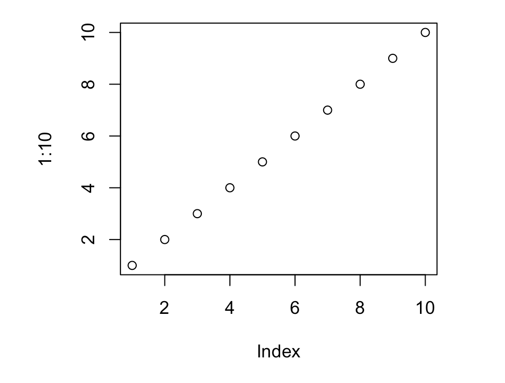
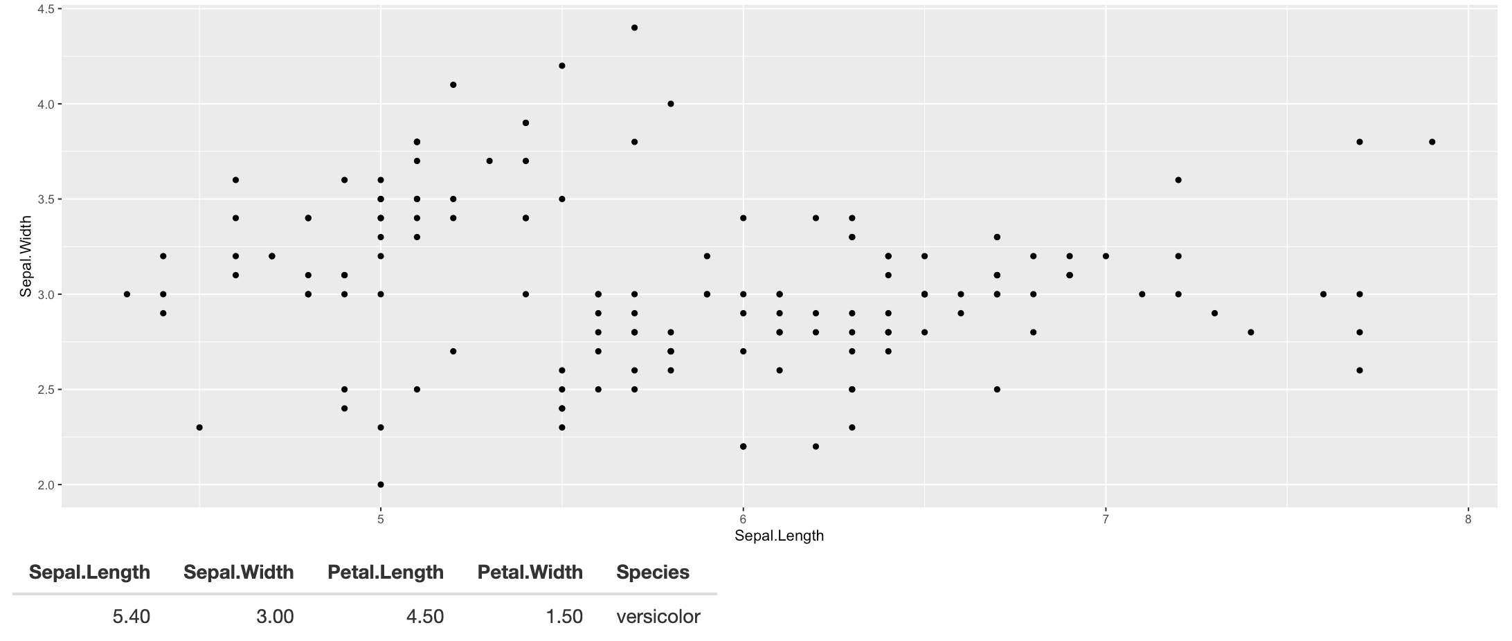
Let’s look at something more interesting. ggplot2 supports interactive mouse inputs, such as click, dblclick, hover, and brush (rectangular select). This time we’re looking at the iris dataset.
library(shiny)
library(ggplot2)

ui <- fluidPage(
  plotOutput("plot", click = "plot_click"),
  tableOutput("data")
)
server <- function(input, output) {
  output$plot <- renderPlot({
    ggplot(iris, aes(x=Sepal.Length, y=Sepal.Width)) +
      geom_point()})

  output$data <- renderTable({
    nearPoints(iris, input$plot_click)
  })
}
shinyApp(ui, server)
Below is just a placeholder image. Try running the code above yourself to see how the mouse click function works.
More plot types can be found on the R Graph Library with helpful example code to get you started. This library focuses on ggplot 2 and tidyverse, so you have already learned what you need to make and modify these!
12.3.6 Images
You can place images or logos in your app! Of course, you also use fluidRow() and column arguments to organize your space with text and images. In this case, we are pointing to an image located at a website.
library("shiny")
ui <- fluidPage(
  mainPanel(
    img(src="https://upload.wikimedia.org/wikipedia/commons/thumb/a/a5/Glazed-Donut.jpg/800px-Glazed-Donut.jpg", align = "center")
  )
)#close fluidPage

server <- function(input, output) {

}#close server
shinyApp(ui, server)
You can also source your image from a directory. Your files should be saved in a folder called ‘www’ inside your working, (or root), directory.
  shinyApp/
     app.R
     www/
        glazedDonut.jpg
        sprinkleDonut.jpg
        cakeDonut.jpg
A simple way to call a locally saved image, such as a logo or banner image, might be this:
library(shiny)

ui <- fluidPage(

    img(src="glazedDonut.jpg", align = "right")

)

server <- function(input, output) {}

shinyApp(ui, server)
However, if we wanted to call those locally saved images from a choice list, our code would need to look like this:
library(shiny)

donuts <- tibble::tribble(
  ~type, ~ id, ~donut,
  "glazed", "glazedDonut","GlazedDonut",
  "sprinkles", "sprinkleDonut", "SprinkleDonut",
  "cake", "cakeDonut", "CakeDonut"
)

ui <- fluidPage(
  selectInput("id", "Pick a donut", choices = setNames(donuts$id, donuts$type)),
  imageOutput("photo")
)
server <- function(input, output, session) {
  output$photo <- renderImage({
    list(
      src = file.path("www", paste0(input$id, ".jpg")),
      contentType = "image/jpeg",
      width = 800,
      height = 650
        )#close list
    }, deleteFile = FALSE)
}#close function

shinyApp(ui, server)Placing many logos across a page can be very tedious and difficult to control. For example, inculding all the logos of universities involved in a research project. It may be easier to combine them all in one image file using an image editor, such as Photoshop or GiMP. Then place that one image on your page.

12.3.7 File uploads
12.3.7.0.1 fileInput()
File uploads and downloads are more complicated types of inputs and outputs. There is a special chapter dedicated to them on the Mastering Shiny webbook here. Loading data, usually in the form of a csv, is a very common need. The following code will upload a csv based on which dataset you’ve chosen from an input menu. However, this code also makes the upload available to the server function and reads it into a table.
library(shiny)

ui <- fluidPage(
    sidebarLayout(
      sidebarPanel(
        fileInput("file1", "Choose a CSV  format File", accept = ".csv"),
        checkboxInput("header", "Header", TRUE)
      ),
      mainPanel(
        tableOutput("contents")
      ) #close mainPanel
    )#close sidebarLayout
  )#close fluidPage

server <- function(input, output) {
    output$contents <- renderTable({
      file <- input$file1
      ext <- tools::file_ext(file$datapath)

      req(file)
      validate(need(ext == "csv", "Please upload a csv format file"))

      read.csv(file$datapath, header = input$header)
    })#close renderTable
  }#close function

shinyApp(ui, server)
12.3.8 Downloads
The download button is a special case and it’s a super useful output for people to download a dataset or whatever, such as a manipulated data from a DataTable. The downloadHandler() function is critical to this working. In this case the downloadHandler() is sending the file named data to the write.csv() function.
ui <- fluidPage(
  downloadButton("downloadData", "Download")
)

server <- function(input, output) {
  # Our dataset
  data <- mtcars

  output$downloadData <- downloadHandler(
    filename = function() {
      paste("data-", Sys.Date(), ".csv", sep=",")
    },
    content = function(file) {
      write.csv(data, file)
    }#close function
  )#close downloadHandler
}#close server function

shinyApp(ui, server)
With other libraries you can also write Excel files, such as with writexl. This version writes to an Excel file.
library(shiny)
library(writexl)


ui <- fluidPage(
    downloadButton("downloadData", "Download")
  )

server <- function(input, output) {
    # Our dataset
    data <- mtcars

    output$downloadData <- downloadHandler(
      filename = function() {
        #paste("data-", Sys.Date(), ".csv", sep="")
        paste("data-", Sys.Date(), ".xlsx")
      },
      content = function(file) {
        #write.csv(data, file)
        writexl::write_xlsx(data, file)
      } #close function
    ) #close downloadHandler
  }#close server function

shinyApp(ui, server)
Next, let’s play with themes.
12.4 Themes
Themes control the styling of the application, unifying colors and fonts, for example. Themes are assigned in the ui(). You can find the shinythemes library here.
library(shinythemes)

ui = fluidPage(theme = shinytheme("cerulean")
  )#close fluidPage

server = function(input,output) {}

shinyApp(ui, server)
Or use the theme picker option until you decide on one!
library(shinythemes)

ui = fluidPage(
    shinythemes::themeSelector()
    )#close fluidPage

server = function(input, output) {}

shinyApp(ui, server)
It is possible to create your own themes, use themes other than Bootstrap, or modify Bootstrap themes to your own aesthetic needs. Mastering Shiny has a brief chapter on themes here, and you can also find more information here on Bootswatch themes. Here is a link for the hex codes or names you’ll need for colors.
You can even start making your own theme by specifying items to be used throughout your app in the ui. Colors are hex or by HTML names. Collections of web safe fonts can be found here. Note how the bslib library is called and the theme is identified in the first part of the page layout. You can find the documentation on bslib here. In this case, the open-source fonts came from Google Fonts.
library(shiny)
library(bslib)

ui <- fluidPage(
  theme = bs_theme(
    bg = "#175d8d",
    fg = "#d5fbfc",
    primary = " #e3fffc",
    base_font = font_google("Atkinson Hyperlegible"),
    code_font = font_google("Roboto Mono")
  ),
  sidebarLayout(
    sidebarPanel(
      fileInput("file1", "Choose a CSV  format File", accept = ".csv"),
      checkboxInput("header", "Header", TRUE)
    ),
    mainPanel(
      tableOutput("contents")
    ) #close mainPanel
  )#close sidebarLayout
)#close fluidPage

server <- function(input, output) {
  output$contents <- renderTable({
    file <- input$file1
    ext <- tools::file_ext(file$datapath)

    req(file)
    validate(need(ext == "csv", "Please upload a csv format file"))

    read.csv(file$datapath, header = input$header)
  })#close renderTable
}#close function

shinyApp(ui, server)
There is also the shiny.semantic library for a different look. You can find the link here.
12.5 Formatting text
12.5.0.1 HTML functions
You can apply HTML equivalent functions in shiny to format your text by creating distinct paragraphs, emphasize text, or change the font or color. The table below shows the shiny function, such as p(), and its HTML equivalent and what is modified.
Table source: https://shiny.rstudio.com/tutorial/written-tutorial/lesson2/
| shiny function | HTML5 equivalent | creates |
|---|---|---|
p |
<p> |
A paragraph of text |
h1 |
<h1> |
A first level header |
h2 |
<h2> |
A second level header |
h3 |
<h3> |
A third level header |
h4 |
<h4> |
A fourth level header |
h5 |
<h5> |
A fifth level header |
h6 |
<h6> |
A sixth level header |
a |
<a> |
A hyper link |
br |
<br> |
A line break (e.g. a blank line) |
div |
<div> |
A division of text with a uniform style |
span |
<span> |
An in-line division of text with a uniform style |
pre |
<pre> |
Text ‘as is’ in a fixed width font |
code |
<code> |
A formatted block of code |
img |
<img> |
An image |
strong |
<strong> |
Bold text |
em |
<em> |
Italicized text |
HTML |
Directly passes a character string as HTML code |
Below is an example with many types of the HTML modifiers.
library(shiny)

ui <- fluidPage(
  titlePanel("My Shiny App"),
  sidebarLayout(
    sidebarPanel(),
    mainPanel(
      h1(" h1() creates a level 1 header."),
      h2(" h2() creates a level 2 header, and so on..."),
      p("Use p() to create a new paragraph. "),
      p("You can apply style to a paragraph using style", style = "font-family: 'times'; font-si16pt"),
      strong("Using strong() bolds text."),
      em("Italics can be applied with em(). "),
      br(),
      p("Use br() to apply a line break."),
      br(),
      code("You can create a code box with code()."),
      div("div creates a container that can apply styles within it using 'style = color:magenta'", style = "color:blue"),
      br(),
      p("span is similar to div but can affect smaller sections",
        span("such as words or phrases", style = "color:purple"),
        "within a paragraph or body of text."),
      h3(p("You can also combine ",
           em(span("HTML", style="color:magenta")),
           "functions."))
    )#close mainPanel
  )#close sidebarLayout
)#close fluidPage
server <- function(input, output) {

}

shinyApp(ui, server)
12.6
12.7 Reactive pages
In this section, we will look at how to make your app respond to inputs and do stuff!
This section is difficult to understand. Take your time with it, and its ok if it doesn’t make sense right away. We’ll be working with this more in class.
12.7.1 Basics of reactivity
Reactivity refers to the ability of an app to recalculate or perform some action when an input is changed. In a non-reactive Shiny app, all calculations are run when the session begins. However, if you want a user to change an input and display a new calculated result, then reactivity in Shiny apps allow only that part of the app to be computed and re-displayed, not the entire app. This is important for making things fast and able to display immediate changes. So, in a sense, reactivity is something that happens in the background, or more accurately, the back-end. But, knowing about it will help you use the following functions successfully.
12.7.1.1 Two different types of programming: imperative and declarative
Imperative programming is like the analysis functions you’ve been running so far in this class. You write a series of commands and R executes them. You see errors if something doesn’t match. The UI layout is imperative. You write code that says where something will be, like a radio button, sidebar text, or text output in the main panel.
Declarative code provides options for the program if conditions are right. So, it will execute the code if conditions are met. This is what we see on the server side function. It is a series of codes that will run if something happens in the UI.
In the context of reactive expressions, all code is run when you start a session and results are stored in the cache. This means that if you move a slider and a new value can be retrieved from that cache, your app will show the result. However, if you move a slider and a new calculated value needs to be shown, this value will not be in your cache. You need some part of the app to calculate and store a new value to be shown. This is where reactivity steps in. Only the part of the code that needs to run, is executed - not the entire app. These declarative bits of code are wrapped in reactive function.
12.7.1.2 Code execution order
Unlike imperative, declarative coding such as in the server, run only when needed. So order is not as important in the server function. However, this can make code very difficult to read for humans as we tend to assume top to bottom. In practice, its best to keep your code human readable. For example, following the order of the ui can be helpful in navigating through the server code.
Data can be very large. To prevent this from slowing down the application, every time a new input is sent to the server function, do as much of your data cleaning and manipulation outside of the ShinyApp as possible. Of course, there are just some situations where this is not possible. But as a general rule, keep it minimal inside the ShinyApp. However, you can run code before the ui and server functions if data needs to be cleaned.
#insert example code
take mtcars and apply some calculation based on existing data, maybe $ to drive 100 miles or km in today.
In the following section, let’s look at two reactive functions commonly found. More information on reactive functions can be found here in the Shiny documentation.
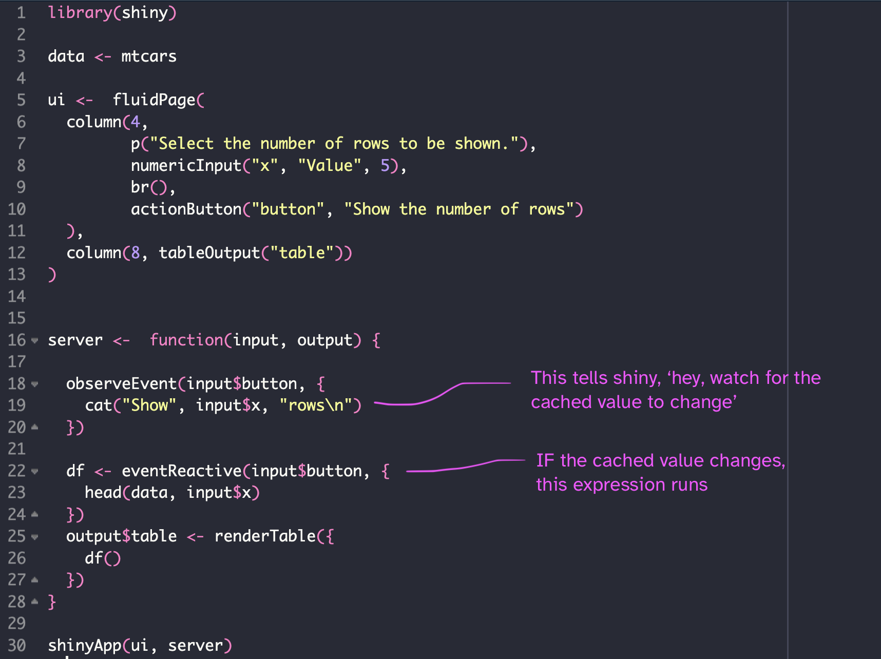
12.7.1.3 observeEvent()
observeEvent() has two arguments: eventExpr and handlerExpr. The first input is the input or expression to take a dependency upon, the second is the code that will be executed.
observeEvent() functions provide the set-up for the eventReactive() by observing the data to check for updates. When updates are noticed, the eventReactive() pulls the new updated data and the HTML updates. Note that the following code changes in the HTML to the webpage with the reactive and also prints something in the console.
12.7.1.4 eventReactive()
When you select the actionButton(), the just the part of the code that needs to run updates what you see. This is great for click events like action buttons, where a user may expect something to occur. Details of the options and examples of eventReactive() and observeEvent() can be found here in the documentation.
Below, we’ve used the example from the documentation to illlustrate basic reactivity. When the app first runs, nothing is displayed as there was no information in the cache for the button ID. Once the button is pressed, the x value is attached to it and the first x rows of data are shown. It does nothing until the cache is updated again when both the x value and the button values have changed.
Reactivity in Shiny is regretably complex. However the two functions above cover the most common ones you’ll see. The free, online book, Mastering Shiny, has 4 chapters dedicated to reactivity in Shiny. For now, when you see observeEvent() and eventReactive() functions in code you are getting from other sources, you should recognize these as reactive parts of the app that will update when some input has been changed.
12.7.1.5 What is session?
Session is an optional argument passed to the server function that enables inputs or outputs related to the current instance of the app to be used. You may see some examples with this. If you see it in a code example, its likely there to pull an input or output that is unique to this instance and do something with it. You can read more in its documentation here.
The session state is used when we need to retrieve some data that has been stored as a result of calculations or inputs from a user’s session. It could be user data, or it could be a file they uploaded that your Shiny app then performed an operation on.
12.8 Summary
Reactivity is different due to the nature of declarative programming. It makes code less complex and providies conditions that could be met, rather than a linear progression of code to be executed. We use reactivity so that people can change inputs and receive different outputs or make external actions happen.
Recognizing reactive functions of eventReactive() and observeEvent() and why its used on the back-end of a Shiny app will help in designing and debugging your code.
You can put code before the Shiny
uicode to reduce calculation time.observeEvent()sets up the reactivity by signaling which inputs the app should look for change.eventReactive()is used to render or provide some action based on the updated input values.
12.9 Wrap up
That was a massive chapter, but this is intended to be used as a reference for you for your future explorations in Shiny. By the end of this you have learned more about many of the Shiny inputs and output functions, how they work together, and an introduction to themes and formatting text. We also introduced reactivity in Shiny which is an important concept as you move forward into more complex interactions. You now have enough information to create and publish web-based applications. Combined with what you have covered in the previous chapters, you are now well prepared to create, modify, calculate, and publish your own research!