Regression is a method used to determine the relationship between a dependent variable (the variable we want to predict) and one or more independent variables (the predictors available to make the prediction). There are a wide variety of regression methods, but in this course we will learn two: the logistic regression, which is used to predict a categorical dependent variable, and the linear regression, which is used to predict a continuous dependent variable.
In this chapter, we focus on the binomial logistic regression (we will refer to it as logistic regression or simply regression in the rest of the chapter), which means that our dependent variable is dichotomous (e.g., yes or no, pass vs fail). Ordinal logistic regression (for ordinal dependent variables) and multinominal logistic regression (for variables with more than 2 categories) are beyond the scope of the course.
9.3 Logistic regression
9.3.1 Logistic function
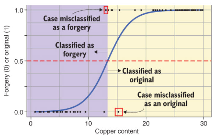
Logistic regression is called this way because it fits a logistic function (an s-shaped curve) to the data to model the relationship between the predictors and a categorical outcome. More specifically, it models the probability of an outcome (the dependent categorical variable) based on the value of the independent variable. Here’s an example:
The model gives us, for each value of the independent variable (Copper content, in this example), the probability (odds) that the painting is an original. The point where the logistic curve reaches .5 (50%) on the y-axis is where the cut-off happens: the model predicts that any painting with a copper content above that point is an original.
9.3.2 Odds
We can convert probabilities into odds by dividing the probability p of the one outcome by the probability of the other outcome, so because there are only two outcomes, then odds = p / 1-p. For example, say we have a bag of 10 balls, 2 red and 8 black. If we draw a ball at random, we have a 8/10 = 80% chance of drawing a black ball. The odds of drawing a black ball are thus 0.8/(1-0.8) = 0.8/0.2 = 4. There is a 4 to 1 chance that we’ll draw a black ball over a red one.
However, the output of the logistic regression model is the natural logarithm of the odds: log odds = ln(p/1-p), so it is not so easily interpreted.
Cumings, Mrs. John Bradley (Florence Briggs Thayer)
female
38
1
0
PC 17599
71.2833
C85
C
3
1
3
Heikkinen, Miss. Laina
female
26
0
0
STON/O2. 3101282
7.9250
NA
S
4
1
1
Futrelle, Mrs. Jacques Heath (Lily May Peel)
female
35
1
0
113803
53.1000
C123
S
5
0
3
Allen, Mr. William Henry
male
35
0
0
373450
8.0500
NA
S
6
0
3
Moran, Mr. James
male
NA
0
0
330877
8.4583
NA
Q
9.4.1.1 Choose a set of predictors (independent variables)
Looking at our dataset, we can identify some variables that we think might affect the probability that a passenger survived. In our model, we will choose Sex, Age, Pclass, and Fare. The SibSp and Parch variables represent, respectively, the combined number of siblings and spouses and the combined number of parents and children a passenger has on board. We will add them together to create a fifth predictor called FamilySize.
data <- data %>%mutate(FamilySize = SibSp + Parch)
We can now remove the variables that we don’t need in our model by selecting the ones we want to keep.
data <- data %>%select(Survived, Sex, Age, Fare, FamilySize, Pclass)head(data) %>%kbl() %>%kable_classic()
Survived
Sex
Age
Fare
FamilySize
Pclass
0
male
22
7.2500
1
3
1
female
38
71.2833
1
1
1
female
26
7.9250
0
3
1
female
35
53.1000
1
1
0
male
35
8.0500
0
3
0
male
NA
8.4583
0
3
9.4.1.2 Set categorical variables as factors
Setting categorical variables as factors is always necessary when fitting regression models in R. In our case there are three: Sex, Survived, and Pclass.
data <- data %>%mutate(Sex =as_factor(Sex),Survived =as_factor(Survived),Pclass =as_factor(Pclass))
9.4.1.3 Dealing with missing data
We can count the number of empty cells for each variable to see if some data is missing. We do this for each variable in the set.
sum(is.na(data$Survived))
[1] 0
sum(is.na(data$Sex))
[1] 0
sum(is.na(data$Age))
[1] 177
sum(is.na(data$Fare))
[1] 0
sum(is.na(data$FamilySize))
[1] 0
sum(is.na(data$Pclass))
[1] 0
Once we have identified that some columns contain missing data, we have two choices. We do nothing and these cases will be left out of the regression model, or we fill the empty cells in some way (this is called imputation). We have many missing values (177 out of 891 observations is quite large) and leaving out these observations could negatively affect the performance of our regression model. Therefore, we will assign the average age for all 177 missing age values, which is a typical imputation mechanism to replace NA values with an estimate based on the available data.
# We use na.rm = TRUE otherwise mean(Age) would return NA due to the missing values.data <- data %>%mutate(Age =replace_na(Age, round(mean(Age, na.rm=TRUE),0)))head(data) %>%kbl() %>%kable_classic()
Survived
Sex
Age
Fare
FamilySize
Pclass
0
male
22
7.2500
1
3
1
female
38
71.2833
1
1
1
female
26
7.9250
0
3
1
female
35
53.1000
1
1
0
male
35
8.0500
0
3
0
male
30
8.4583
0
3
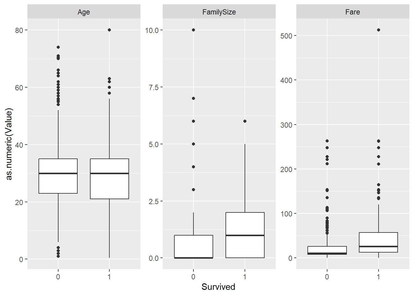
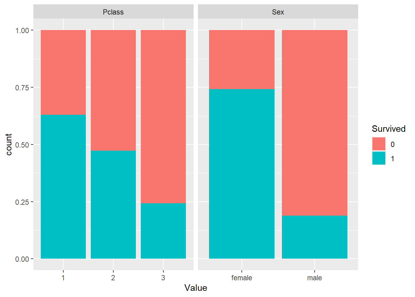
9.4.2 Visualizing the relationships
To explore the relationship between variables. we can visualize the distribution of independent variable values for each value of the dependent variable. We can use box plots or violin plots for continuous independent variables and bar charts for the categorical variables. To make the process faster, let’s briefly untidy the data and use the gather() function to create key-value pairs for each observation of the dependent variable.
data_untidy <-gather(data, key ="Variable", value ="Value",-Survived) # Creates key-value pairs for all columns except Survivehead(data_untidy) %>%kbl() %>%kable_classic()
Survived
Variable
Value
0
Sex
male
1
Sex
female
1
Sex
female
1
Sex
female
0
Sex
male
0
Sex
male
We can now easily create box plots for all our independent variables and outcome.
The following code generates our logistic regression model using the glm() function (glm stands for general linear model). The syntax is gml(predicted variable ~ predictor1 + predictor2 + preductor3..., data, family) where data is our dataset and the family is the type of regression model we want to create. In our case, the family is binomial.
model <-glm(Survived ~ Sex + Age + Fare + FamilySize + Pclass,data = data,family = binomial)
9.4.3.1 Model summary
Now that we have created our model, we can look at the coefficients (estimates) which tell us about the relationship between our predictors and the predicted variable. The Pr(>|z|) column represents the p-value, which determines whether the effect observed is statistically significant. It is common to use 0.05 as the threshold for statistical significance, so all the effects in our model are statistically significant (p < 0.05) except for the fare (p > 0.05).
As we mentioned above, the coefficients produced by the model are log odds, which are difficult to interpret. We can convert them to odds ratio, which are easier to interpret. This can be done with the exp() function. We can now see that according to our model, female passengers were 16 times more likely to survive than male passengers.
The confidence intervals are an estimation of the precision odds ratio. In the example below, We use a 95% confidence interval which means that we are 95% of our estimated coefficients for a predictor are between the 2.5th percentile and the 97.5th percentile (the two values reported in the tables). If we were using a sample to make claims about a population, which does not really apply here due to the unique case of the titanic, we could then think of the confidence interval as indicating a 95% probability that the true coefficient for the entire population is situated in between the two values.
First we add to our data the probability that the passenger survived as calculated by the model.
data <-tibble(data,Probability = model$fitted.values)head(data) %>%kbl() %>%kable_classic()
Survived
Sex
Age
Fare
FamilySize
Pclass
Probability
0
male
22
7.2500
1
3
0.1025490
1
female
38
71.2833
1
1
0.9107566
1
female
26
7.9250
0
3
0.6675927
1
female
35
53.1000
1
1
0.9153720
0
male
35
8.0500
0
3
0.0810373
0
male
30
8.4583
0
3
0.0968507
Then we obtain the prediction by creating a new variable called prediction and setting the value to 1 if the calculated probability of survival is greater than 50% and 0 otherwise.
data <- data %>%mutate(Prediction =if_else(Probability >0.5,1,0))head(data) %>%kbl() %>%kable_classic()
Survived
Sex
Age
Fare
FamilySize
Pclass
Probability
Prediction
0
male
22
7.2500
1
3
0.1025490
0
1
female
38
71.2833
1
1
0.9107566
1
1
female
26
7.9250
0
3
0.6675927
1
1
female
35
53.1000
1
1
0.9153720
1
0
male
35
8.0500
0
3
0.0810373
0
0
male
30
8.4583
0
3
0.0968507
0
Then we can print a table comparing the model’s prediction to the real data.
Finally, we can calculate how well our model fits the data (how good was it at predicting the independent variable) by testing, for each passenger in the dataset, whether the prediction matched the actual outcome for that passenger. Because that test gives TRUE (1) or FALSE (0) for every row of the dataset, calculating the mean of the test results gives us the percentage of correct predictions, which in our case is about 80.5%.
mean(data$Survived == data$Prediction)
[1] 0.8047138
9.5 Summary
In this chapter we introduced the logistic regression model as a useful tool to predict a dichotomous categorical variable based on one or multiple predictors that can be either categorical or continuous. The R scripts provided will work with any dataset provided that they are in a tidy format. So you now have everything you need to try to predict categorical outcomes in all kinds of scenarios and with all kinds of data.
9.6 Lab
For this week’s lab, your task is to build a logistic regression model on a dataset of your choice. I encourage you to use the dataset that you will be using for your individual project, if it contains a dichotomous variable that you can try to predict using other variables in your dataset.